Variational inference methods in Bayesian inference and machine learning are techniques which are involved in approximating intractable integrals. Most of the machine learning techniques involves finding the point estimates (Maximum likelihood estimation (MLE), Maximum a posteriori estimate (MAP)) of the latent variables, parameters which certainly do not account for any uncertainty. For taking account of uncertainty in point estimates, an entire posterior distribution over the latent variables and parameters is approximated.
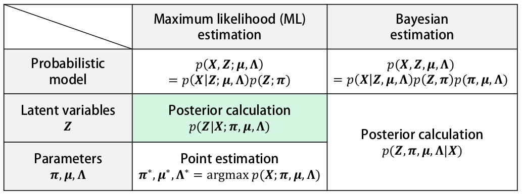
For approximation of posterior distribution, which involves intractable integrals variational inference methods are applied for making the calculation tractable (having some kind of close form mathematically !!) i.e. which does not involve calculation of marginal distribution of the observed variables P(X).

The marginalisation over Z to calculate P(X) is intractable, because of the search space of Z is combinatorially large, thus we seek an approximation, using variational distribution Q(Z) with it’s own variational parameters.
Variational Inference as an Optimisation problem
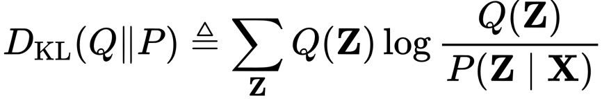
Since we are trying to approximate a true posterior distribution p(Z|X) with Q(Z), a good choice of measure for measuring the dissimilarity between the true posterior and approximated posterior is Kullback–Leibler divergence (KL-divergence),
which is basically expectation of difference in log of two probability distribution with respect to approximated distribution. Considering KL divergence as an optimisation function, it needs to be minimised with respect to variational parameters of the variational distribution Q(Z). Since calculating KL divergence itself involves the calculation of posterior distribution P(Z|X), the calculation of dissimilarity in-terms of KL divergence needs to be expressed where we come across Evidence lower bound (ELBO). The above expression KL divergence can be written in terms of ELBO as

in which log evidence log P(X) is constant with respect to Q(Z), maximising the term L(Q) (Evidence lower bound) minimises KL divergence. By choosing an appropriate choice of Q(Z), L(Q) becomes maximizable and tractable to compute.
Mean field approximation
The mean field approximation assumes that all the hidden variables are independent of each other, which simplifies the joint distribution of hidden variables as the product of marginal distribution of each hidden variable.
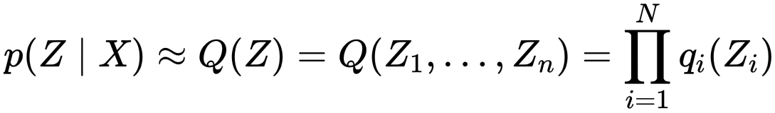
where N is the no. of the hidden variables. It can be shown that best distribution qⱼ(Zⱼ) for maximising ELBO can be estimated as

which is expectation of log joint probability distribution of observed and latent variables taken over variables which do not include Zⱼ. This type above equations can be simplified into functions of hyper-parameters of the prior distribution over the latent variable and expectation of the latent variables which is not being calculated. These type of equation create circular between the parameters of the distribution over the variables being calculated and expectation of variables not being calculated, this section of circular dependencies will be more clear in the following section. This circular dependence of distribution of parameters of the variational distribution suggest an iterative update procedure same as Expectation-Maximisation algorithm.
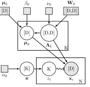
Variational inference in Gaussian mixture model